How to Use Python Pandas and SQL Together for Data Analysis

For all the tasks related to data science and machine learning, the most important thing that defines how a model will perform depends on how good our data is. Python Pandas and SQL are among the powerful tools that can help in extracting and manipulating data efficiently. By combining these two together, data analysts can perform complex analysis on even large datasets. In this article, we’ll explore how you can combine Python Pandas with SQL to enhance the quality of data analysis.

Pandas and SQL: Overview

Before using Pandas and SQL together. First, we’ll go through Pandas and SQL is capable of and their key features.

What is Pandas?

Pandas is a software library written for Python programming language for data manipulation and analysis. It offers operations for manipulating tables, data structures, and time series data.

Key Features of Pandas

• Pandas DataFrames allow us to work with structured data. 
• It offers different functionalities like sorting, grouping, merging, reshaping, and filtering data.
• It is efficient in handling missing data values.

Learn More: The Ultimate Guide to Pandas For Data Science!

What is SQL?

SQL stands for Structured Query Language, which is used for extracting, managing, and manipulating relational databases. It is useful in handling structured data by incorporating relations among entities and variables. It allows for inserting, updating, deleting, and managing the stored data in tables. 

Key Features of SQL

• It provides a robust way for querying large datasets.
• It allows the creation, modification, and deletion of database schemas.
• The syntax of SQL is optimized for efficient and complex query operations like JOIN, GROUPBY, ORDER BY, HAVING, using sub-queries.

Learn More: SQL For Data Science: A Beginner’s Guide!

Why Combine Pandas with SQL?

Using Pandas and SQL together makes the code more readable and, in certain cases, easier to implement. This is true for complex workflows, as SQL queries are much clearer and easier to read than the equivalent Pandas code. Moreover, most of the relational data originates from databases, and SQL is one of the main tools to deal with relational data. This is one of the main reasons why working professionals like data analysts and data scientists prefer to integrate their functionalities.

How Does pandasql Work?

To combine SQL queries with Pandas, one needs a common bridge between these two, so to overcome this problem, ‘pandasql’ comes into the picture. Pandasql allows you to run SQL queries directly within Pandas. In this way, we can seamlessly use the SQL syntax without leaving the dynamic Pandas environment.

Installing pandasql

The first step to using Pandas and SQL together is to install pandasql into our environment.

pip install pandasql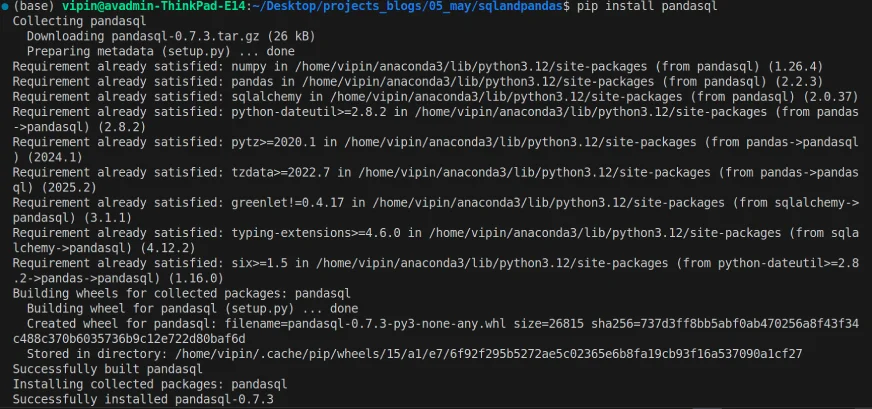

Once the installation is complete, we can import the pandasql into our code and use it to execute the SQL queries on Pandas DataFrame.

Running SQL Queries in Pandas

Once the installation is over, we can import the pandasql and start exploring it.

import pandas as pd
import pandasql as psql

# Create a sample DataFrame
data = {'Name': ['Alice', 'Bob', 'Charlie'], 'Age': [25, 30, 35]}
df = pd.DataFrame(data)

# SQL query to select all data
query = "SELECT * FROM df"
result = psql.sqldf(query, locals())
result

Let’s break down the code

• pd.DataFrame will convert the sample data into a tabular format.
• query (SELECT * FROM df) will select everything in the form of the DataFrame. 
• psql.sqldf(query, locals()) will execute the SQL query on the DataFrame using the local scope.

Data Analysis with pandasql

Once all the libraries are imported, it’s time to perform the data analysis using pandasql. The below section shows a few examples of how one can enhance the data analysis by combining Pandas and SQL. To do this:

Step 1: Load the Data

# Required libraries
import pandas as pd
import pandasql as ps
import plotly.express as px
import ipywidgets as widgets
# Load the dataset
car_data = pd.read_csv("cars_datasets.csv")
car_data.head()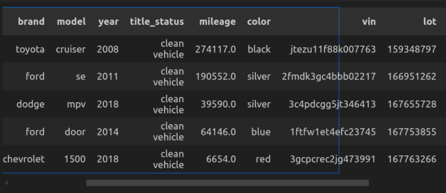

Let’s break down the code

• Importing the necessary libraries: pandas for handling data, pandasql for querying the DataFrames, plotly for making interactive plots.
• pd.read_csv(“cars_datasets.csv”) to load the data from the local directory.
• car_data.head() will display the top 5 rows.

Step 2: Explore the Data

In this section, we’ll try to get familiar with data by exploring things like the names of columns, the data type of the features, and whether the data has any null values or not.

1. Check the column names.

# Display column names
column_names = car_data.columns
column_names
"""
Output:
Index(['Unnamed: 0', 'price', 'brand', 'model', 'year', 'title_status',
      'mileage', 'color', 'vin', 'lot', 'state', 'country', 'condition'],
     dtype="object")
""”

2. Identify the data type of the columns.

# Display dataset info
car_data.info()
"""
Ouput:

RangeIndex: 2499 entries, 0 to 2498
Data columns (total 13 columns):
#   Column        Non-Null Count  Dtype 
---  ------        --------------  ----- 
0   Unnamed: 0    2499 non-null   int64 
1   price         2499 non-null   int64 
2   brand         2499 non-null   object
3   model         2499 non-null   object
4   year          2499 non-null   int64 
5   title_status  2499 non-null   object
6   mileage       2499 non-null   float64
7   color         2499 non-null   object
8   vin           2499 non-null   object
9   lot           2499 non-null   int64 
10  state         2499 non-null   object
11  country       2499 non-null   object
12  condition     2499 non-null   object
dtypes: float64(1), int64(4), object(8)
memory usage: 253.9+ KB
"""

3. Check for Null values.

# Check for null values
car_data.isnull().sum()


"""Output:
Unnamed: 0      0
price           0
brand           0
model           0
year            0
title_status    0
mileage         0
color           0
vin             0
lot             0
state           0
country         0
condition       0
dtype: int64
"""

Step 3: Analyze the Data

Once we have loaded the dataset into the workflow. Now we will begin by performing data analysis.

Examples of Data Analysis with Python Pandas and SQL

Now let’s try using pandasql to analyze the above dataset by running some of our queries.

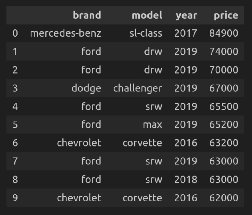
Query 1: Selecting the 10 Most Expensive Cars

Let’s first find the top 10 most expensive cars from the entire dataset.

def q(query):
   return ps.sqldf(query, {'car_data': car_data})
q("""
SELECT brand, model, year, price
FROM car_data
ORDER BY price DESC
LIMIT 10
""")

Let’s break down the code

• q(query) is a custom function that executes the SQL query on the DataFrame.
• The query iterates over the complete dataset and selects columns such as brand, model, year, price, and then sorts them by price in descending order.

Query 2: Average Price by Brand

Here we’ll find the average price of cars for each brand.

def q(query):
   return ps.sqldf(query, {'car_data': car_data})

q("""
SELECT brand, ROUND(AVG(price), 2) AS avg_price
FROM car_data
GROUP BY brand
ORDER BY avg_price DESC""")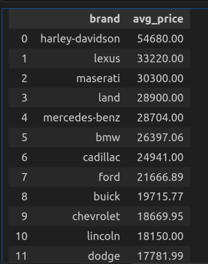

Let’s break down the code

• Here, the query uses AVG(price) to calculate the average price for each brand and uses round, round off the resultant to 2 decimals.
• And GROUPBY will group the data by the car brands and sort it by using the AVG(price) in descending order.

Query 3: Cars Manufactured After 2015

Let’s make a list of the cars manufactured after 2015.

def q(query):
   return ps.sqldf(query, {'car_data': car_data})

q("""
SELECT *
FROM car_data
WHERE year > 2015
ORDER BY year DESC
""")

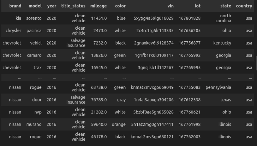
Let’s break down the code

• Here, the query selects all the car manufacturers after 2015 and orders them in descending order.

Query 4: Top 5 Brands by Number of Cars Listed

Now let’s find the total number of cars produced by each brand.

def q(query):
   return ps.sqldf(query, {'car_data': car_data})

q("""
SELECT brand, COUNT(*) as total_listed
FROM car_data
GROUP BY brand
ORDER BY total_listed DESC
LIMIT 5
""")

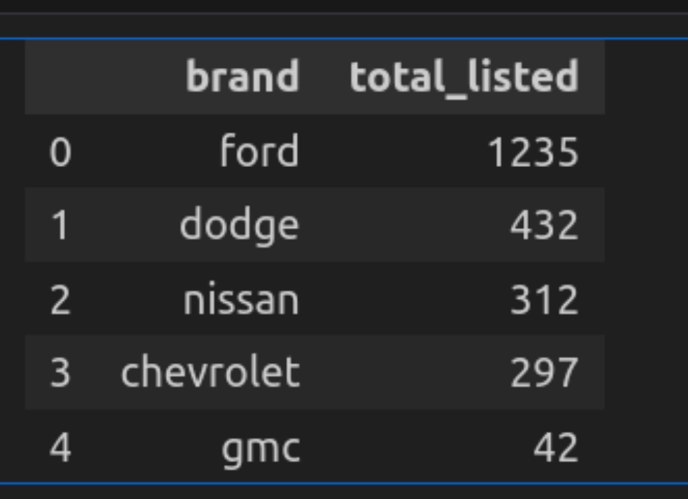
Let’s break down the code

• Here the query counts the total number of cars by each brand using the GROUP BY operation.
• It lists them in descending order and uses a limit of 5 to pick out only the top 5.

Query 5: Average Price by Condition

Let’s see how we can group the cars based on a condition. Here, the condition column shows the time when the listing was added or how much time is left. Based on that, we can categorize the cars and get their average pricing.

def q(query):
   return ps.sqldf(query, {'car_data': car_data})

q("""
SELECT condition, ROUND(AVG(price), 2) AS avg_price, COUNT(*) as listings
FROM car_data
GROUP BY condition
ORDER BY avg_price DESC
""")

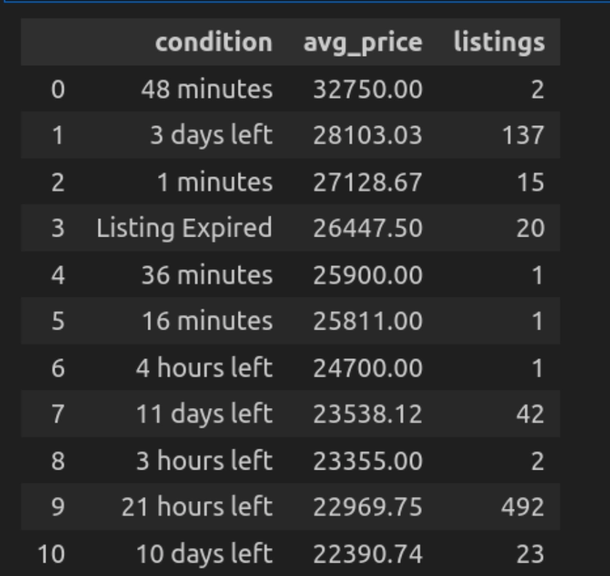
Let’s break down the code

• Here, the query groups the cars on condition (such as new or used) and calculates the price using AVG(Price).
• Order them in descending order to show the most expensive cars first.

Query 6: Average Mileage and Price by Brand

Here we’ll find the average mileage of the cars for each brand and their average price. 

def q(query):
   return ps.sqldf(query, {'car_data': car_data})

q("""
SELECT brand,
      ROUND(AVG(mileage), 2) AS avg_mileage,
      ROUND(AVG(price), 2) AS avg_price,
      COUNT(*) AS total_listings
FROM car_data
GROUP BY brand
ORDER BY avg_price DESC
LIMIT 10
""")

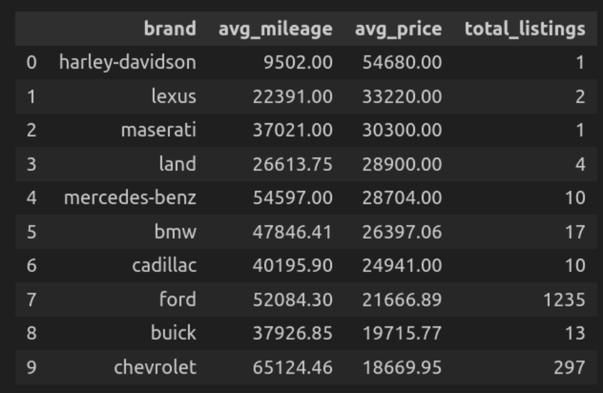
Let’s break down the code

• Here, the query groups the cars using brand and calculates their average mileage and average price, and counts the total number of listings of each brand in that group.
• Order them in descending order by price.

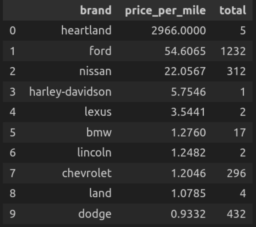
Query 7: Price per Mileage Ratio for Top Brands

Now let’s sort the top brands based on their calculated mileage ratio i.e. the average price per mile of the cars for each brand.

def q(query):
   return ps.sqldf(query, {'car_data': car_data})

q("""
SELECT brand,
      ROUND(AVG(price/mileage), 4) AS price_per_mile,
      COUNT(*) AS total
FROM car_data
WHERE mileage > 0
GROUP BY brand
ORDER BY price_per_mile DESC
LIMIT 10
""")

Let’s break down the code

• Here query calculates the price per mileage for each brand and then shows cars by each brand with that specific price per mileage. In descending order by price per mile.

Query 8: Average Car Price by Area

Here we’ll find and plot the number of cars of each brand in a particular city. 

state_dropdown = widgets.Dropdown(
   options=car_data['state'].unique().tolist(),
   value=car_data['state'].unique()[0],
   description='Select State:',
   layout=widgets.Layout(width="50%")
)

def plot_avg_price_state(state_selected):
   query = f"""
       SELECT brand, AVG(price) AS avg_price
       FROM car_data
       WHERE state="{state_selected}"
       GROUP BY brand
       ORDER BY avg_price DESC
   """
   result = q(query)
   fig = px.bar(result, x='brand', y='avg_price', color="brand",
                title=f"Average Car Price in {state_selected}")
   fig.show()

widgets.interact(plot_avg_price_state, state_selected=state_dropdown)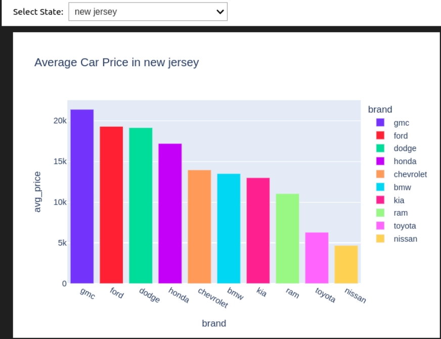

Let’s break down the code

• State_dropdown creates a dropdown to select the different US states from the data and allows the user to select a state.
• plot_avg_price_state(state_selected) executes the query to calculate the average price per brand and gives a bar chart using plotly.
• widgets.interact() links the dropdown with the function so the chart can update on its own when the user selects a different state.

For the notebook and the dataset used here, please visit this link.

Limitations of pandasql

Even though pandasql offers many efficient functionalities and a convenient way to run SQL queries with Pandas, it also has some limitations. In this section, we’ll explore these limitations and try to figure out when to rely on traditional Pandas or SQL, and when to use pandasql.

• Not compatible with large datasets: While we run the pandasql query creates a copy of the data in memory before complete execution of the current query. This method of executing the over queries dealing with large datasets can lead to high memory usage and slow execution.
• Limited SQL Features:  pandasql supports many basic SQL features, but it fails to fully implement all the advanced features like subqueries, complex joins, and window functions.
• Compatibility with Complex Data: pandas works well with tabular data. While working with complex data, such as nested JSON or multi-index DataFrames, it fails to provide the desired results.

Conclusion

Using Pandas and SQL together significantly improves the data analysis workflow. By leveraging pandasql, one can seamlessly run SQL queries in the DataFrames. This helps those who are familiar with SQL and want to work in Python environments. This integration of Pandas and SQL combines the flexibility of both and opens up new possibilities for data manipulation and analysis. With this, one can enhance the ability to tackle a wide range of data challenges. However, it’s important to consider the limitations of pandasql as well, and explore other approaches when dealing with large and complex datasets.

Hello! I’m Vipin, a passionate data science and machine learning enthusiast with a strong foundation in data analysis, machine learning algorithms, and programming. I have hands-on experience in building models, managing messy data, and solving real-world problems. My goal is to apply data-driven insights to create practical solutions that drive results. I’m eager to contribute my skills in a collaborative environment while continuing to learn and grow in the fields of Data Science, Machine Learning, and NLP.