 “Follow the data. Update your beliefs.”
We like the idea of applying iterative Bayesian thinking to how we test hypotheses and conduct UX research.
The idea is simple, but modern Bayesian math can be opaque and hard to understand.
We have questions about how well Bayesian analysis works relative to frequentist analysis. We are also intrigued by the possibility of Bayesian thinking in UX research.
The best way to understand how to apply Bayesian thinking and math to UX is to match the original Bayesian examples from hundreds of years ago to modern problems in UX. And it starts with urns.
Statistics, Probability, and Urns
Statistics is abstract. Probability is hard to understand. And conditional probability is harder still.
One way to make probability more concrete is through cards, dice, and coins. We’re not trying to make people compulsive gamblers. Historically, however, many of our modern formulas come from games of chance. If you can understand how to win a card game or avoid a costly mistake at the roulette table, you tend to pay more attention.
And this is where Thomas Bayes’ famous essay on the logic of updating beliefs from observed outcomes (e.g., successes and failures) comes into play. This work was published after he died in 1763, a reminder that sometimes the private scraps of an idea can publicly change the world.
While cards and dice work for teaching basic probability, conditional probability is often clearer with a different classic tool: the urn problem. In its simplest form, two urns contain different proportions of colored balls. After drawing a sample, the task is to determine which urn most likely produced it.
The advantage of urn problems is flexibility. Unlike coins (two sides), dice (six sides), or cards (fixed suits and ranks), urns allow probabilities to vary in ways that make Bayesian comparisons easier to illustrate.
We modified an example from Cowles’ excellent book, Statistics in Psychology: An Historical Perspective, to demonstratethe use of Bayesian analysis to assess the relative likelihood of competing urn hypotheses (and who noted on p. 75, “Traditionally, writers on Bayes make heavy use of ‘urn problems’”).
For the example depicted in Figure 1, suppose you have a sample of 20 balls where 18 are green and 2 are red. Is this sample more likely to have come from an urn with 90% green balls (Urn A) or one with 78% green balls (Urn B)?
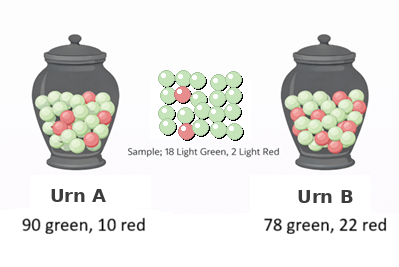
Figure 1: Depiction of a classical urn problem.
Before we go through the math to compare the likelihoods, let’s update the narrative. After all, UX researchers don’t work with urns. We work with users.
From Balls in Urns to Users Checking Out
In our earlier article, we introduced Bayesian thinking using a checkout completion example with 20 participants, 18 who successfully completed the task and two who failed.
So instead of asking which urn produced a sample of green and red balls, let’s ask a question more relevant to UX research: Is this checkout experience performing at a historical level, or is it consistent with a more aspirational goal?
That’s the same math, just with a better context.
Instead of trying to figure out which urn a sample of balls came from, we want to know which of two possible completion rates is more likely.
- Historical Completion Rate of 78% (Hypothesis H): This comes from a historical average with an overall 78% completion.
- Aspirational Completion Rate of 90% (Hypothesis A): It’s aspirational because in this hypothetical example, we have a reason to believe (or at least hope) the checkout flow is better than average.
Because the observed percentage of success from the sample is exactly 90%, this seems more consistent with the aspirational hypothesis. But let’s work through the math using Bayes’ theorem.
Comparing these two hypotheses, the exact probability of the aspirational 90% hypothesis is:
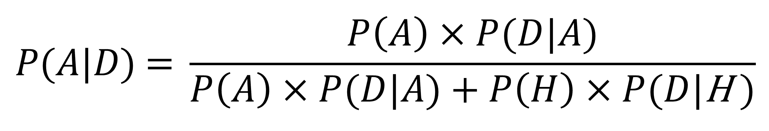
where:
P(D|A) is the probability of getting this sample (the data, D) if the aspirational hypothesis is true.
P(D|H) is the probability of getting this sample if the historical hypothesis is true.
P(A) is our expected (prior) probability that the aspirational hypothesis is true.
P(H) is our expected (prior) probability that the historical hypothesis is true.
P(A|D) is the conditional probability of the aspirational hypothesis given the sample.
Using binomial probabilities, P(D|A) is (0.9)18 × (0.1)2 = 0.0015 and P(D|H) is (0.78)18 × (0.22)2 = 0.00055. Assuming we have no prior belief favoring either hypothesis (so P(A) = P(H) = 0.5), we get:

which equals 0.00075/(0.00075 + 0.000275) = 0.00075/0.001025 = 0.732 (73.2%). Because P(A|D) + P(H|D) = 1, P(H|D) = 0.268 (26.8%).
We conclude there is a substantial probability that the historical hypothesis might be true (26.8% isn’t anywhere near 0%), but the aspirational hypothesis is 2.7 times more likely.
Summary and Discussion
In this article, we extended a classic Bayesian urn exercise to illustrate one way to apply Bayesian analysis to a UX research context.
We showed how you can use a relatively simple version of Bayes’ theorem to compare the likelihoods of two hypotheses from observed completion rate data.
Even though we couldn’t say with certainty that either hypothesis was implausible, the data were clearly a better fit for the aspirational hypothesis.
But this leaves more questions:
- Is comparing two hypotheses in this way a better approach than just using a confidence (or credibility) interval, or using binomial tests to compare the sample against the two benchmarks (78%, 90%)?
- How do we come up with a solid prior? We avoided that question in this example by using the principle of indifference (setting both priors to 0.5). But what if we had a good reason to believe that the historical value of 78% should receive more (or less) weight in the calculation? How much could that change the posterior belief (P(A|D)) and consequent decisions?
We’ll address these questions in future articles.
Note that we aren’t recommending this specific method in UX analysis. One of our primary goals in this article is to illustrate the mechanics of Bayesian analysis with simple algebra and binomial probabilities. The downside of this is that we had to assign specific prior probabilities rather than following the current practice of using beta distributions for priors. This does not, however, affect the logic of the discussion.